Tensor Rank Hierarchy & Coordinate Transformation Studio - Rank-0 Scalars, Rank-1 Vectors, and Rank-2 Tensors under Coordinate Rotation (Trace & Determinant Invariants)
Interactive Physics Ready
Click "Run Code" to launch simulation and interactive parameter sliders.
Mathematical Problem Formulation
Theoretical Background & Explanation
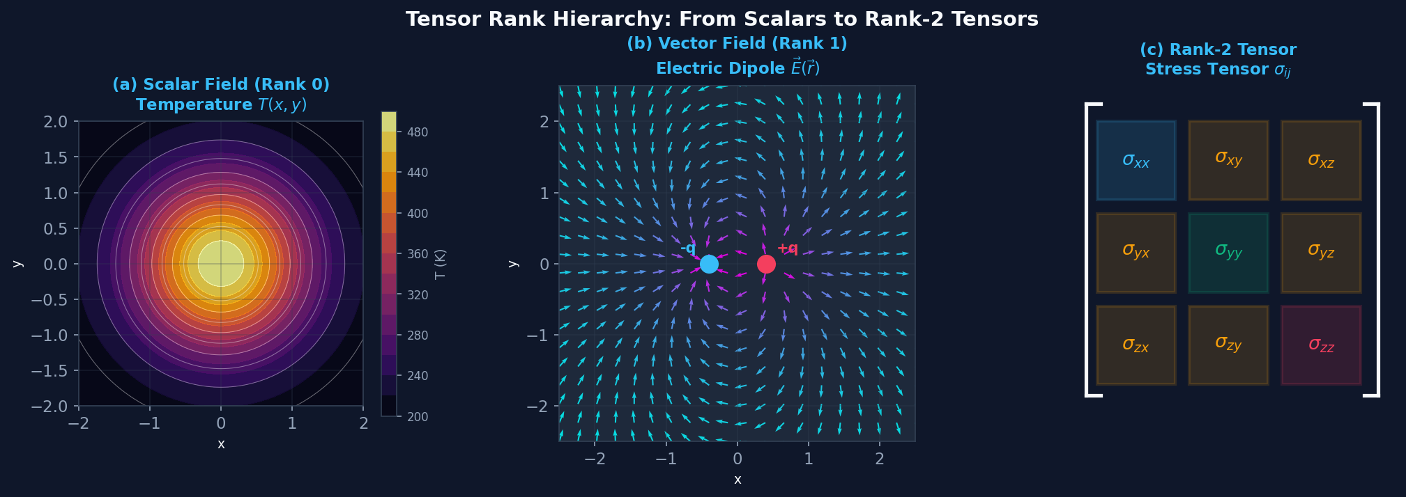
Figure 2.1: Tensor Rank Hierarchy: (a) Rank-0 scalar field (temperature $T$), (b) Rank-1 vector field (electric dipole $\vec{E}$), (c) Rank-2 tensor transformation quadric ($x^T T x = 1$) under frame rotation showing strict invariance of trace and determinant.
What is a Tensor in Physics?
A tensor is a geometric, coordinate-independent physical entity that establishes a linear multilinear relationship between geometric vectors. Crucially, a tensor is defined by how its numerical components transform under a change of coordinate basis. Physical laws must be form-invariant (covariant) under coordinate transformations.
1. The Tensor Rank Hierarchy
In an $N$-dimensional space (typically $N=3$ in Newtonian physics or $N=4$ in Special Relativity), the rank of a tensor determines how many indices it carries and how many components describe it ($N^{\text{rank}}$):
| Rank | Entity | Components ($N=3$) | Transformation Law | Physical Examples |
|---|---|---|---|---|
| 0 | Scalar | $3^0 = 1$ | $S' = S$ | Temperature $T$, Mass $m$, Energy $E$, Pressure $p$ |
| 1 | Vector | $3^1 = 3$ | $v'_i = R_{ij} v_j$ | Displacement $\vec{r}$, Velocity $\vec{v}$, Force $\vec{F}$, Electric Field $\vec{E}$ |
| 2 | Dyad / Matrix | $3^2 = 9$ | $T'_{ij} = R_{im} R_{jn} T_{mn}$ | Stress $[\sigma]$, Strain $[\varepsilon]$, Inertia $[I]$, Metric $[g]$, Conductivity $[K]$ |
| 4 | 4th-Order Tensor | $3^4 = 81$ | $C'_{ijkl} = R_{ia} R_{jb} R_{kc} R_{ld} C_{abcd}$ | Elastic Stiffness Tensor $C_{ijkl}$, Riemann Curvature $R^\rho_{\ \sigma\mu\nu}$ |
2. Transformation Law for Rank-2 Tensors
Consider an orthogonal rotation matrix $R$ between coordinate frame $S$ and rotated frame $S'$, satisfying $R R^T = \mathbb{I}$. The transformation of a rank-2 Cartesian tensor in index notation and matrix notation is:
Notice that each tensor index transforms with one factor of the rotation matrix $R$.
3. Fundamental Tensor Invariants
While individual matrix components $T_{ij}$ change with coordinate rotation, certain scalar combinations remain completely invariant:
In the interactive studio above, rotate the coordinate frame to see that the trace $\mathrm{Tr}(T)$ and determinant $\det(T)$ are constant regardless of $\theta$!
Physics Problem - Anisotropic Thermal Conductivity & Directional Heat Flux Vector under Arbitrary Coordinate Rotation
Interactive Physics Ready
Click "Run Code" to launch simulation and interactive parameter sliders.
Mathematical Problem Formulation
Theoretical Background & Explanation
Problem Statement: Anisotropic Heat Flow
In isotropic materials, heat flows strictly anti-parallel to the thermal gradient ($\vec{q} = -k \nabla T$). However, in anisotropic crystals (such as graphite, quartz, or bismuth telluride composites), the thermal conductivity is a rank-2 symmetric tensor $[K]$. Given principal conductivities $k_1$ and $k_2$ along orthogonal crystal axes, determine the heat flux vector $\vec{q}$ and its angular deviation $\delta$ from $-\nabla T$ when the crystal axis is inclined at an angle $\theta$ relative to an applied horizontal gradient.
1. Fourier's Law in General Tensor Form
Fourier's law for an anisotropic medium is expressed in index notation as:
From the Onsager reciprocal relations, the thermal conductivity tensor is strictly symmetric: $K_{ij} = K_{ji}$.
2. Coordinate Rotation of the Conductivity Tensor
In the crystal's principal coordinate frame, $[K]$ is diagonal:
Rotating the crystal by angle $\theta$ relative to the laboratory $x$-axis via rotation matrix $R(\theta)$:
3. Heat Flux Components and Angular Deflection
For an applied gradient $-\nabla T = (G_0, 0)^T$ along the laboratory $x$-axis:
Key Insights:
• If $\theta = 0^\circ$ or $90^\circ$, $q_y = 0$, so $\vec{q} \parallel -\nabla T$ (flow along principal symmetry directions).
• For intermediate angles, $q_y \neq 0$, generating a sideways transverse heat current!
• The maximum deflection occurs at $\cos 2\theta = -(k_1 - k_2)/(k_1 + k_2)$, with $\sin\delta_{\max} = \frac{k_1 - k_2}{k_1 + k_2}$.