Curvilinear Coordinate Systems - 3D Visualization of Cartesian, Cylindrical, and Spherical Polar Coordinate Surfaces, Scale Factors, and Local Basis Vectors
Interactive Physics Ready
Click "Run Code" to launch simulation and interactive parameter sliders.
Mathematical Problem Formulation
Theoretical Background & Explanation
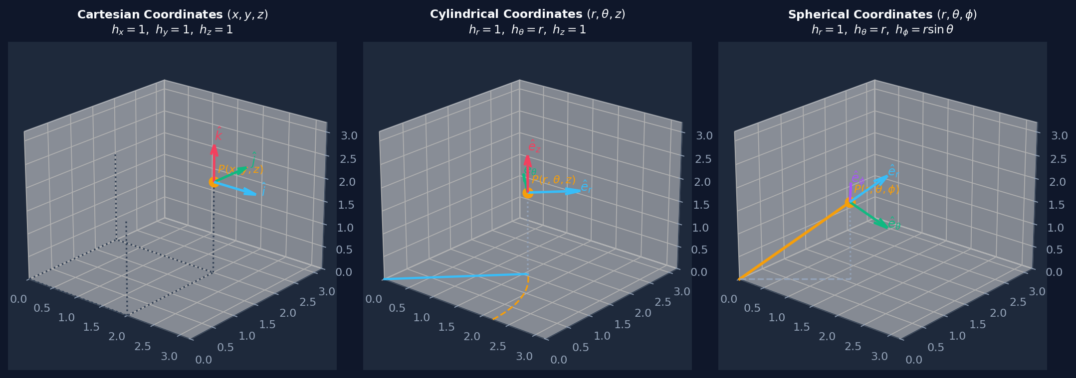
Figure 5.1: Orthogonal Curvilinear Coordinate Systems: (Left) Cartesian $(x,y,z)$ with fixed basis vectors, (Middle) Cylindrical $(r,\theta,z)$ with scale factors $h_r=1, h_\theta=r, h_z=1$, (Right) Spherical polar $(r,\theta,\phi)$ with coordinate surfaces (sphere, cone, half-plane) and position-dependent unit vectors.
General Theory of Orthogonal Curvilinear Coordinates
Let $(u_1, u_2, u_3)$ be generalized coordinates related to Cartesian coordinates by transformation equations $x = x(u_1,u_2,u_3), y = y(u_1,u_2,u_3), z = z(u_1,u_2,u_3)$. The position vector is $\vec{r} = x\hat{i} + y\hat{j} + z\hat{k}$.
1. Scale Factors (Metric Coefficients) & Unit Vectors
The tangent vector along the coordinate curve $u_i$ is $\vec{b}_i = \frac{\partial \vec{r}}{\partial u_i}$. The scale factors $h_i$ measure the physical arc length traversed per unit increment of coordinate $u_i$:
The squared differential arc length and differential volume element are:
2. Comparison Table: Cartesian, Cylindrical & Spherical
| Coordinate System | Coordinates $(u_1, u_2, u_3)$ | Scale Factors $(h_1, h_2, h_3)$ | Volume Element $dV$ |
|---|---|---|---|
| Cartesian | $(x, y, z)$ | $h_x=1, \ h_y=1, \ h_z=1$ | $dx \, dy \, dz$ |
| Cylindrical | $(r, \theta, z)$ | $h_r=1, \ h_\theta=r, \ h_z=1$ | $r \, dr \, d\theta \, dz$ |
| Spherical Polar | $(r, \theta, \phi)$ | $h_r=1, \ h_\theta=r, \ h_\phi=r\sin\theta$ | $r^2\sin\theta \, dr \, d\theta \, d\phi$ |
3. Master Differential Operators in Curvilinear Coordinates
Problem - Gradient, Divergence, and Laplacian in Spherical Coordinates for an Electrostatic Dipole Potential
Interactive Physics Ready
Click "Run Code" to launch simulation and interactive parameter sliders.
Mathematical Problem Formulation
Theoretical Background & Explanation
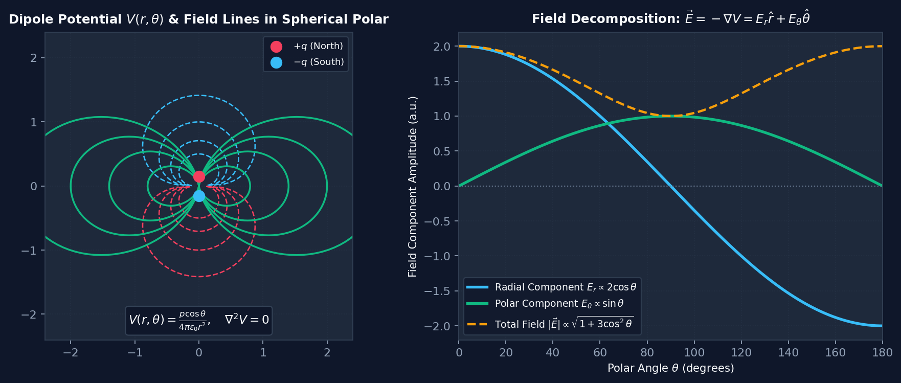
Figure 5.2: Physical Dipole in Spherical Polar Coordinates: (Left) Electric dipole potential contours $V(r,\theta) = \text{const}$ (dashed) and field streamlines $r = r_0 \sin^2\theta$ (solid), (Right) Analytical decomposition into orthogonal spherical components $E_r \propto 2\cos\theta$ and $E_\theta \propto \sin\theta$.
Physics Problem Statement
The electrostatic potential of an electric dipole of moment $p$ oriented along the $z$-axis is given in spherical polar coordinates $(r, \theta, \phi)$ by:
$$V(r, \theta) = \frac{p \cos\theta}{4\pi\epsilon_0 r^2}, \quad r > 0$$
Tasks:
1. Use the spherical gradient operator to calculate the electric field vector $\vec{E}(r, \theta) = -\nabla V$.
2. Prove by direct differentiation in spherical coordinates that $V$ satisfies Laplace's Equation $\nabla^2 V = 0$ everywhere outside the origin ($r > 0$).
3. Derive the differential equation of the electric field lines and prove they form the closed curves $r = r_0 \sin^2\theta$.
1. Spherical Gradient & Electric Field Components
In spherical polar coordinates, the gradient of a scalar field is: $$\nabla V = \frac{\partial V}{\partial r}\hat{e}_r + \frac{1}{r}\frac{\partial V}{\partial \theta}\hat{e}_\theta + \frac{1}{r\sin\theta}\frac{\partial V}{\partial \phi}\hat{e}_\phi$$ Evaluating the partial derivatives for $V(r, \theta) = \frac{p\cos\theta}{4\pi\epsilon_0 r^2}$:
The resultant total electric field is: $$\vec{E} = \frac{p}{4\pi\epsilon_0 r^3}\left( 2\cos\theta\hat{e}_r + \sin\theta\hat{e}_\theta \right), \qquad |\vec{E}| = \frac{p}{4\pi\epsilon_0 r^3}\sqrt{1 + 3\cos^2\theta}$$
2. Proof of Laplace's Equation in Spherical Coordinates
The Laplacian operator in spherical coordinates for an azimuthally symmetric potential ($V = V(r,\theta)$) is:
Evaluating the radial term: $$\frac{\partial V}{\partial r} = -\frac{2p\cos\theta}{4\pi\epsilon_0 r^3} \implies r^2 \frac{\partial V}{\partial r} = -\frac{2p\cos\theta}{4\pi\epsilon_0 r} \implies \frac{\partial}{\partial r}\left( r^2 \frac{\partial V}{\partial r} \right) = +\frac{2p\cos\theta}{4\pi\epsilon_0 r^2}$$ $$\text{Radial Term} = \frac{1}{r^2}\left( +\frac{2p\cos\theta}{4\pi\epsilon_0 r^2} \right) = +\frac{2p\cos\theta}{4\pi\epsilon_0 r^4}$$ Evaluating the polar angular term: $$\frac{\partial V}{\partial \theta} = -\frac{p\sin\theta}{4\pi\epsilon_0 r^2} \implies \sin\theta \frac{\partial V}{\partial \theta} = -\frac{p\sin^2\theta}{4\pi\epsilon_0 r^2}$$ $$\frac{\partial}{\partial\theta}\left( \sin\theta \frac{\partial V}{\partial\theta} \right) = -\frac{2p\sin\theta\cos\theta}{4\pi\epsilon_0 r^2}$$ $$\text{Angular Term} = \frac{1}{r^2\sin\theta}\left( -\frac{2p\sin\theta\cos\theta}{4\pi\epsilon_0 r^2} \right) = -\frac{2p\cos\theta}{4\pi\epsilon_0 r^4}$$ Adding both terms together:
3. Differential Equation of Electric Field Lines
Along an electric field line, the differential displacement vector $d\vec{r} = dr\hat{e}_r + r d\theta\hat{e}_\theta$ is collinear with $\vec{E}$:
Integrating both sides: $$\ln r = 2\ln(\sin\theta) + \text{constant} \implies r = r_0 \sin^2\theta$$ This yields the characteristic closed dipole loops shown in the interactive simulation!