2D/3D Vector Field Divergence & Flux Density Visualizer - Point Sources, Sinks, Dipoles, and Incompressible Solenoidal Flow
Interactive Physics Ready
Click "Run Code" to launch simulation and interactive parameter sliders.
Mathematical Problem Formulation
Theoretical Background & Explanation
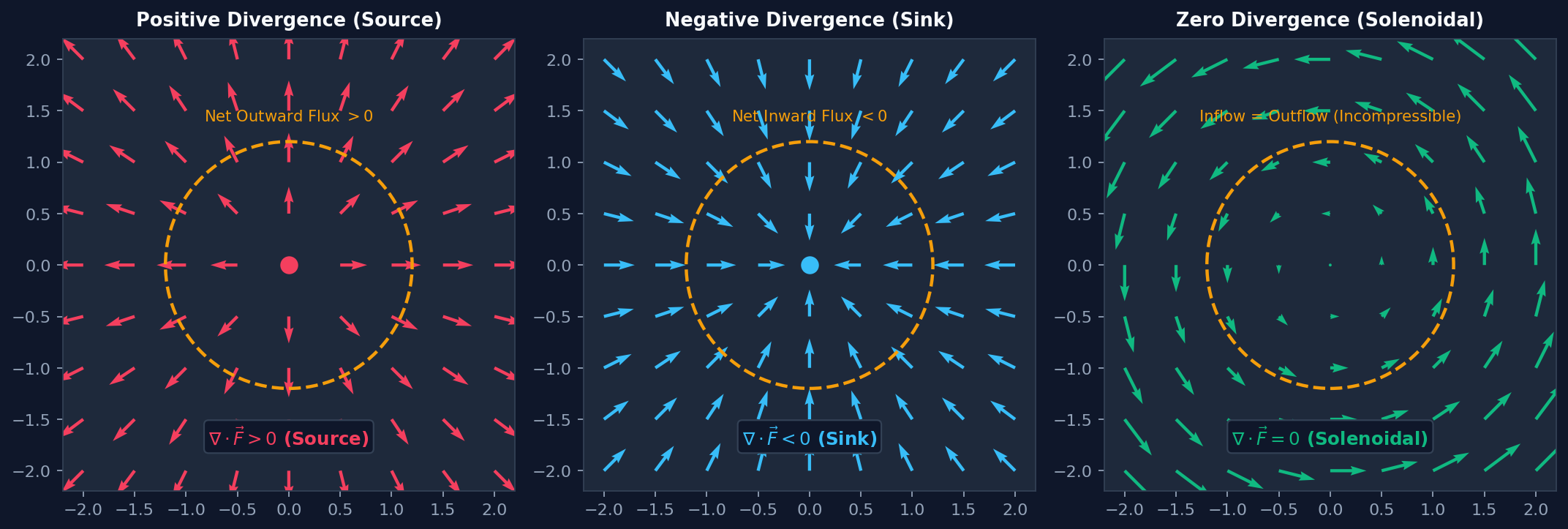
Figure 2.1: Physical Meaning of Divergence: (Left) Positive divergence $\nabla \cdot \vec{F} > 0$ acting as a field source with net outward flux, (Middle) Negative divergence $\nabla \cdot \vec{F} < 0$ acting as a field sink with net inward flux, (Right) Zero divergence $\nabla \cdot \vec{F} = 0$ representing solenoidal/incompressible flow with equal inflow and outflow.
The Divergence Operator ($\nabla \cdot \vec{F}$)
The divergence of a vector field $\vec{F}(x,y,z)$ is a scalar field quantifying the net outward flux of the vector field per unit volume expanding away from an infinitesimal point: $$\nabla \cdot \vec{F} = \lim_{\Delta V \to 0} \frac{1}{\Delta V} \oiint_{\Delta S} \vec{F} \cdot d\vec{S}$$
1. Rectangular Cartesian Formulation
Taking the inner product between the spatial del operator $\nabla = \hat{i}\frac{\partial}{\partial x} + \hat{j}\frac{\partial}{\partial y} + \hat{k}\frac{\partial}{\partial z}$ and the vector field $\vec{F} = F_x \hat{i} + F_y \hat{j} + F_z \hat{k}$:
Consider an infinitesimal rectangular box of dimensions $\Delta x \times \Delta y \times \Delta z$. The net outward flux through the two faces perpendicular to the $x$-axis is: $$\Delta \Phi_x = \left[ F_x\left(x + \frac{\Delta x}{2}, y, z\right) - F_x\left(x - \frac{\Delta x}{2}, y, z\right) \right] \Delta y \Delta z \approx \frac{\partial F_x}{\partial x} \Delta x \Delta y \Delta z$$ Summing over all three pairs of faces and dividing by $\Delta V = \Delta x \Delta y \Delta z$ rigorously produces the Cartesian formula above.
2. Physical Classification of Vector Fields
The sign of $\nabla \cdot \vec{F}$ classifies physical behavior across all transport phenomena:
• $\nabla \cdot \vec{F} > 0$ (Source): Field lines originate here. Positive electric charge in electrostatics ($\nabla \cdot \vec{E} = \rho / \epsilon_0$), or fluid thermal expansion.
• $\nabla \cdot \vec{F} < 0$ (Sink): Field lines terminate here. Negative electric charge, fluid suction drain, or mass condensation.
• $\nabla \cdot \vec{F} = 0$ (Solenoidal / Incompressible): Field lines never begin or end; they form continuous closed loops or extend from $-\infty$ to $+\infty$.
• Examples of Solenoidal Fields: Magnetic induction $\nabla \cdot \vec{B} = 0$ (Gauss's law for magnetism; no magnetic monopoles exist), and incompressible fluid velocity $\nabla \cdot \vec{v} = 0$ (equation of continuity with constant fluid density).
Problem - Verification of Gauss's Law for a Non-Uniform Spherically Symmetric Charge Distribution
Interactive Physics Ready
Click "Run Code" to launch simulation and interactive parameter sliders.
Mathematical Problem Formulation
Theoretical Background & Explanation
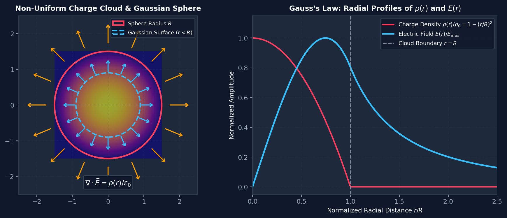
Figure 2.2: Gauss's Law & Divergence in Non-Uniform Spherical Charge: (Left) Cross-sectional volume density and outward electric field quivers with concentric Gaussian sphere $r < R$, (Right) Radial profiles of charge density $\rho(r)$ and continuous electric field $E(r)$ smoothly transitioning across the boundary $r = R$.
Physics Problem Statement
A spherically symmetric cosmic dust cloud of radius $R$ contains a non-uniform volume charge density given by:
$$\rho(r) = \begin{cases} \rho_0 \left( 1 - \frac{r^2}{R^2} \right), & r \le R \ 0, & r > R \end{cases}$$
where $\rho_0$ is the peak charge density at the center $r=0$.
Tasks:
1. Calculate the total charge $Q_{\text{tot}}$ enclosed by the entire cloud.
2. Use the integral form of Gauss's Law $\oiint \vec{E} \cdot d\vec{S} = Q_{\text{enc}} / \epsilon_0$ to determine the electric field $\vec{E}(r)$ everywhere ($r \le R$ and $r > R$).
3. Verify that the differential divergence $\nabla \cdot \vec{E} = \frac{1}{r^2}\frac{d}{dr}(r^2 E_r)$ yields identically $\rho(r) / \epsilon_0$.
1. Total Enclosed Charge Calculation
Integrating the volume density in spherical coordinates with radial shells of volume $dV = 4\pi r^2 dr$:
2. Electric Field via Gauss's Law
By spherical symmetry, the electric field is purely radial: $\vec{E} = E(r)\hat{r}$. Over a concentric Gaussian sphere of radius $r$:
$$\oiint_S \vec{E} \cdot d\vec{S} = E(r) \cdot 4\pi r^2 = \frac{Q_{\text{enc}}(r)}{\epsilon_0}$$
• Inside the Cloud ($r \le R$):
• Outside the Cloud ($r > R$):
$$E_{\text{out}}(r) = \frac{Q_{\text{tot}}}{4\pi\epsilon_0 r^2} = \frac{2\rho_0 R^3}{15\epsilon_0 r^2}$$
3. Differential Verification of Divergence
Applying the spherical divergence formula to $E_{\text{in}}(r)$:
This completes the exact analytical and numerical proof connecting integral Gauss's law with Maxwell's 1st differential equation $\nabla \cdot \vec{E} = \rho / \epsilon_0$!