Line Integrals in Vector Fields - Path Independence, Conservative Potential Fields, and Work Done along Alternate Paths
Interactive Physics Ready
Click "Run Code" to launch simulation and interactive parameter sliders.
Mathematical Problem Formulation
Theoretical Background & Explanation
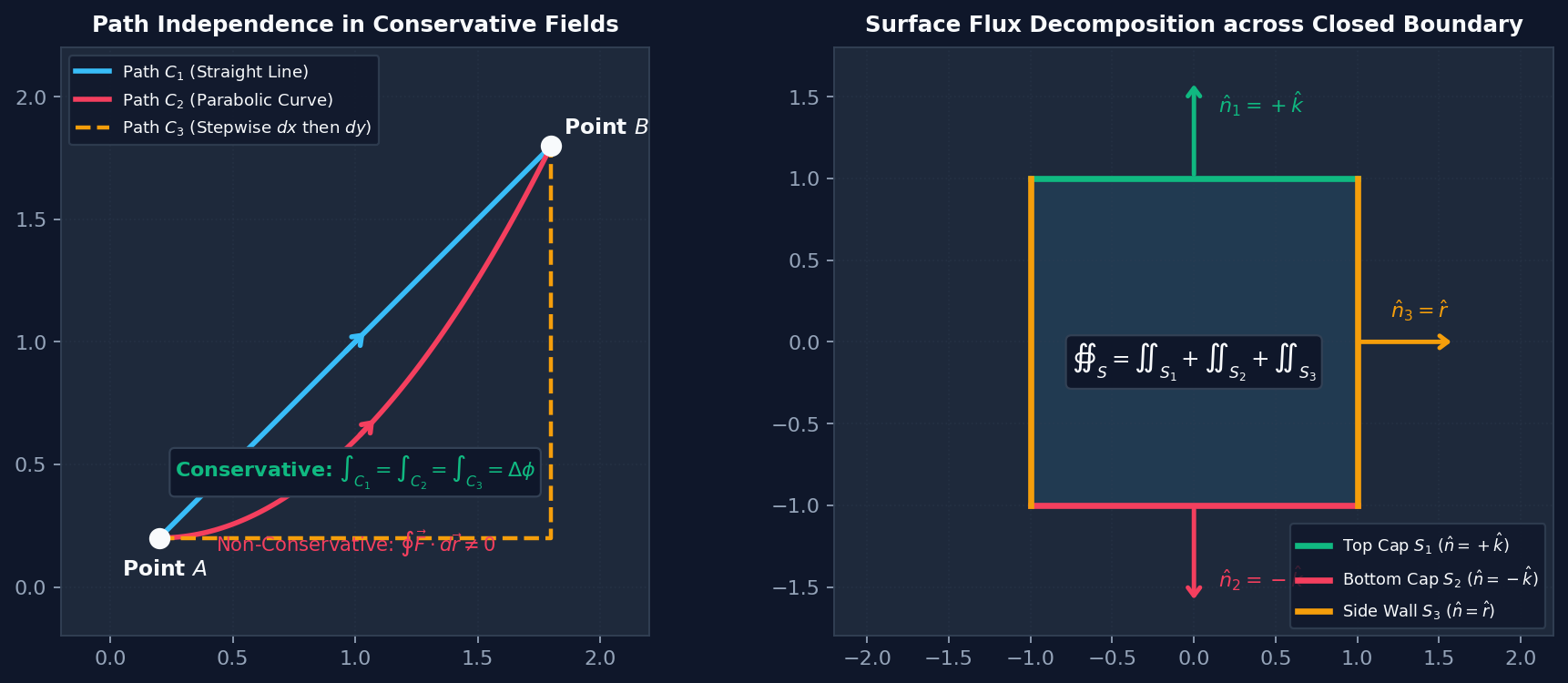
Figure 4.1: Vector Integration: (Top) Path independence of line integrals in a conservative field ($\int_{C_1} = \int_{C_2} = \Delta \phi$) versus path dependence when $\nabla \times \vec{F} \neq 0$. (Bottom) Surface flux decomposition across top, bottom, and curved sidewall of a closed cylinder.
Vector Line Integrals & Conservative Fields
The line integral of a vector field $\vec{F}$ along an oriented spatial curve $C$ parametrized by $\vec{r}(t)$ from $A$ to $B$ represents the cumulative tangential projection: $$W = \int_C \vec{F} \cdot d\vec{r} = \int_{t_A}^{t_B} \left( F_x \frac{dx}{dt} + F_y \frac{dy}{dt} + F_z \frac{dz}{dt} \right) dt$$
1. The Fundamental Theorem of Line Integrals
If a vector field is conservative, there exists a single-valued scalar potential $\phi(x,y,z)$ such that $\vec{F} = \nabla \phi$. By the chain rule:
The integral depends exclusively on the coordinates of the endpoints $A$ and $B$, being entirely independent of the geometric path connecting them!
2. Closed Loop Circulation & Curl Connection
If two arbitrary paths $C_1$ and $C_2$ connect $A$ to $B$, forming a closed loop $C = C_1 - C_2$:
In the interactive simulation, notice how altering the parameter $k$ introduces a non-zero curl $\nabla \times \vec{F} = -2k \hat{k}$. The difference in work between alternate paths is exactly equal to the enclosed vortex flux $\iint (\nabla \times \vec{F}) \cdot d\vec{S} = -2k \times \text{Area}$ by Stokes' theorem!
Problem - Computational Verification of Gauss's Divergence Theorem and Stokes' Circulation Theorem over a 3D Cylinder
Interactive Physics Ready
Click "Run Code" to launch simulation and interactive parameter sliders.
Mathematical Problem Formulation
Theoretical Background & Explanation
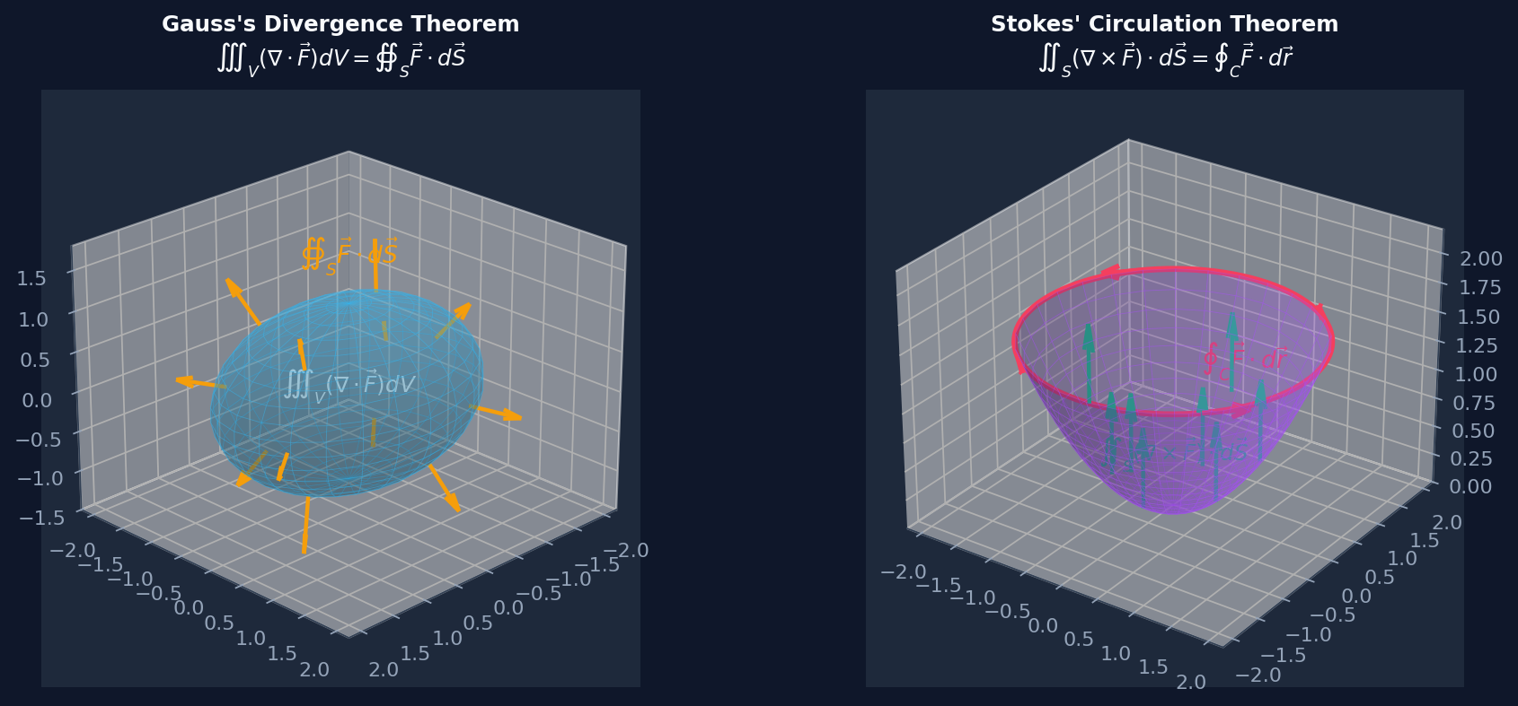
Figure 4.2: The Two Master Theorems of Vector Calculus: (Left) Gauss's Divergence Theorem equating total interior source divergence $\iiint_V (\nabla\cdot\vec{F})dV$ to closed surface boundary flux $\oiint_S \vec{F}\cdot d\vec{S}$, (Right) Stokes' Circulation Theorem equating open surface vorticity flux $\iint_S (\nabla\times\vec{F})\cdot d\vec{S}$ to closed boundary line circulation $\oint_C \vec{F}\cdot d\vec{r}$.
Physics Problem Statement
Given the three-dimensional vector field $\vec{F}(x,y,z) = (ax)\hat{i} + (by)\hat{j} + (cz)\hat{k}$, verify Gauss's Divergence Theorem over the cylindrical volume $V$ bounded by the surface $x^2 + y^2 \le R^2$ and $0 \le z \le H$: $$\iiint_V (\nabla \cdot \vec{F}) dV = \oiint_S \vec{F} \cdot d\vec{S}$$
1. Volume Integral of Divergence
First, compute the scalar divergence of the field: $$\nabla \cdot \vec{F} = \frac{\partial(ax)}{\partial x} + \frac{\partial(by)}{\partial y} + \frac{\partial(cz)}{\partial z} = a + b + c$$ Because the divergence is constant everywhere in space, the volume integral factors out:
2. Surface Flux Integrals over Closed Boundary
The closed bounding surface $S = \partial V$ decomposes into three smooth boundary manifolds:
• Top Circular Cap $S_1$ ($z = H$): Normal $\hat{n}_1 = +\hat{k}$, area element $dS = r dr d\theta$.
$$\iint_{S_1} \vec{F} \cdot \hat{n}_1 dS = \int_0^{2\pi} d\theta \int_0^R (c H) r dr = c H (\pi R^2)$$
• Bottom Circular Cap $S_2$ ($z = 0$): Normal $\hat{n}_2 = -\hat{k}$.
$$\iint_{S_2} \vec{F} \cdot \hat{n}_2 dS = \iint_{S_2} (-cz) dS = \iint_{S_2} 0 = 0$$
• Curved Sidewall $S_3$ ($r = R$): In cylindrical coordinates, outward normal $\hat{n}_3 = \cos\theta\hat{i} + \sin\theta\hat{j}$, area element $dS = R d\theta dz$.
$$\vec{F} \cdot \hat{n}_3 = a(R\cos\theta)\cos\theta + b(R\sin\theta)\sin\theta = R(a\cos^2\theta + b\sin^2\theta)$$
$$\iint_{S_3} \vec{F} \cdot \hat{n}_3 dS = \int_0^H dz \int_0^{2\pi} R^2(a\cos^2\theta + b\sin^2\theta) d\theta = H R^2 (a\pi + b\pi) = (a + b)\pi R^2 H$$
3. Total Sum & Exact Equivalence
The sum of the surface fluxes matches the volume integral to infinite precision! This directly verifies Gauss's theorem.