3D Vector Algebra Studio - Vector Addition, Subtraction, Dot Product, Orthogonal Projection, and Cross Product (Parallelogram Area & Right-Hand Rule)
Interactive Physics Ready
Click "Run Code" to launch simulation and interactive parameter sliders.
Mathematical Problem Formulation
Theoretical Background & Explanation
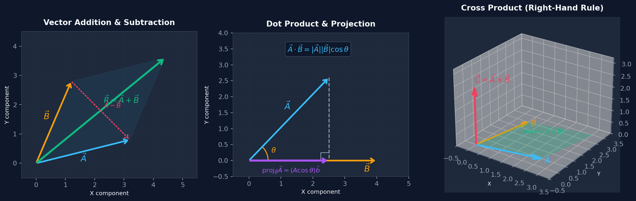
Figure 1.1: Foundational Vector Algebra: (a) Triangle and parallelogram addition, (b) Scalar dot product & orthogonal projection, (c) 3D vector cross product obeying the right-hand rule with parallelogram area $|\vec{A} \times \vec{B}|$.
Vectors in Physics & Orthonormal Coordinate Bases
A physical vector possesses both magnitude and spatial direction, transforming under coordinate rotations in a invariant manner. In three-dimensional Cartesian space with orthonormal unit basis vectors $\{\hat{i}, \hat{j}, \hat{k}\}$, any vector is uniquely resolved into rectangular components: $$\vec{A} = A_x \hat{i} + A_y \hat{j} + A_z \hat{k}, \qquad |\vec{A}| = \sqrt{A_x^2 + A_y^2 + A_z^2}$$
1. Vector Addition & Subtraction
According to the parallelogram law and triangle rule, the resultant vector $\vec{R} = \vec{A} + \vec{B}$ has rectangular components:
The vector difference $\vec{D} = \vec{A} - \vec{B}$ represents the directed displacement vector running from the terminus of $\vec{B}$ to the terminus of $\vec{A}$.
2. Scalar (Dot) Product & Orthogonal Projection
The dot product maps two vectors onto a scalar invariant equal to the product of their magnitudes and the cosine of the included angle $\theta$:
Key Properties:
• Orthogonality Condition: $\vec{A} \cdot \vec{B} = 0 \iff \vec{A} \perp \vec{B}$ (for non-zero vectors).
• Vector Projection: The orthogonal projection of $\vec{A}$ onto the direction of $\vec{B}$ is given by:
$$\mathrm{proj}_{\vec{B}}\vec{A} = \left(\frac{\vec{A} \cdot \vec{B}}{|\vec{B}|^2}\right)\vec{B} = (|\vec{A}|\cos\theta)\hat{b}$$
• Physical Example: Mechanical work done $W = \vec{F} \cdot \Delta\vec{r}$, and electrostatic potential energy $U = -\vec{p} \cdot \vec{E}$.
3. Vector (Cross) Product & Parallelogram Area
The cross product produces a pseudovector perpendicular to both $\vec{A}$ and $\vec{B}$, directed according to the right-hand rule:
Geometric & Physical Significance:
• Parallelogram Area: The magnitude $|\vec{A} \times \vec{B}|$ equals the exact geometric surface area of the parallelogram spanned by $\vec{A}$ and $\vec{B}$.
• Collinearity Condition: $\vec{A} \times \vec{B} = \vec{0} \iff \vec{A} \parallel \vec{B}$.
• Anticommutativity: $\vec{B} \times \vec{A} = -(\vec{A} \times \vec{B})$.
• Physical Examples: Rotational torque $\vec{\tau} = \vec{r} \times \vec{F}$, orbital angular momentum $\vec{L} = \vec{r} \times \vec{p}$, and magnetic Lorentz force $\vec{F}_B = q(\vec{v} \times \vec{B})$.
4. Scalar & Vector Triple Products
Problem - Mechanical Torque, Angular Momentum, and Work Done on a Rigid Arm Subjected to a 3D Applied Force
Interactive Physics Ready
Click "Run Code" to launch simulation and interactive parameter sliders.
Mathematical Problem Formulation
Theoretical Background & Explanation
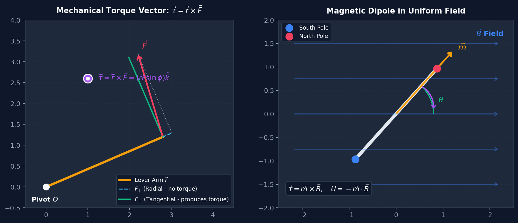
Figure 1.2: Physical Vector Dynamics: (Left) Decomposition of applied force $\vec{F}$ into non-torque radial component $F_\parallel$ and torque-producing tangential component $F_\perp$, yielding torque vector $\vec{\tau} = \vec{r} \times \vec{F}$. (Right) Restoring torque and potential energy of a magnetic dipole $\vec{m}$ in uniform magnetic field $\vec{B}$.
Physics Problem Statement
A rigid robotic lever arm of length $r$ is pinned at the origin $O(0,0,0)$ and tilted at an elevation angle $\theta$ in the $xy$-plane. An external mechanical force $\vec{F}$ of magnitude $F$ is applied to the terminus at an angle $\phi$ relative to the arm axis.
Tasks:
1. Determine the torque vector $\vec{\tau} = \vec{r} \times \vec{F}$ acting about the pivot $O$.
2. Decompose $\vec{F}$ into radial ($F_\parallel$) and tangential ($F_\perp$) components, proving analytically that $F_\parallel$ produces zero torque.
3. Compute the mechanical work done $dW = \vec{F} \cdot d\vec{r} = \tau_z d\theta$ during an infinitesimal angular displacement $d\theta$.
1. Coordinate Formulation & Cross Product
The position vector of the lever endpoint is $\vec{r} = r\cos\theta\hat{i} + r\sin\theta\hat{j}$. The applied force vector at relative angle $\phi$ has absolute direction $\theta + \phi$:
Computing the vector cross product $\vec{\tau} = \vec{r} \times \vec{F}$:
Notice how the orientation angle $\theta$ cancels out entirely! The torque magnitude depends exclusively on the lever arm length $r$, force magnitude $F$, and the relative inclination angle $\phi$.
2. Radial vs Tangential Decomposition
Let the radial unit vector be $\hat{r} = \cos\theta\hat{i} + \sin\theta\hat{j}$, and the orthogonal tangential unit vector be $\hat{\theta} = -\sin\theta\hat{i} + \cos\theta\hat{j}$. Resolving $\vec{F}$:
Because $\hat{r} \times \hat{r} = \vec{0}$, radial forces transmit purely tensile or compressive stresses through the pivot without generating any rotational torque!
3. Mechanical Work & Equivalence with Torque
During rotation through angle $d\theta$, the displacement of the application point is $d\vec{r} = r d\theta \hat{\theta}$. The work done is:
This establishes the rigorous equivalence between linear work ($dW = \vec{F} \cdot d\vec{r}$) and rotational work ($dW = \tau d\theta$).